

Clearly worried that the market would get the “wrong” idea, and having obviously listened to the cacophony of analysts and pundits who have spent the three weeks since the September funding squeeze warning that the announcement of “organic” balance sheet growth to replenish apparently “scarce” reserves needed to be carefully communicated to avoid triggering the “classic” QE trade, Jerome Powell was very explicit on Tuesday in remarks to economists in Denver.
“The time is now upon us” to increase the Fed’s holdings of securities, Powell said, employing a needlessly dramatic turn of phrase in prepared remarks for “Trucks and Terabytes: Integrating the ‘Old’ and ‘New’ Economies”, at the 61st Annual Meeting of the NABE in Colorado.
“I want to emphasize that growth of our balance sheet for reserve management purposes should in no way be confused with the large-scale asset purchase programs that we deployed after the financial crisis”, Powell said, relishing the one time when his patented “plain English” is actually the appropriate cadence.
Read more: If ‘QE-Lite’ Reignites Classic QE Trade, Fade It, Goldman Says
In the wake of the money market “chaos” that unfolded ahead of the September FOMC meeting, it became readily apparent that the Fed needed to grow the balance sheet or else introduce a standing repo facility to address funding stress in a sustainable way.
Unable to cobble together a plan in time (although the factors that conspired to create the September repo madness were known in advance, the severity of the squeeze caught most observers off guard), the Fed instead opted to conduct overnight and term repos as a stopgap into and through the October meeting.
Tuesday’s comments from Powell in Denver sound like the unofficial announcement of what will be official later this month.
“Neither the recent technical issues nor the purchases of Treasury bills we are contemplating to resolve them should materially affect the stance of monetary policy”, he went on to say, adding that when it comes to rates, there is no preset course.
Projections, estimates and predictions vary around the exact parameters and time table on new Fed balance sheet expansion (“QE-Lite”, affectionately). The quote above clearly indicates that the Fed views September’s dramatics as stemming in no small part from America’s public debt trajectory and the knock-on effect to markets.
Generally speaking, analysts see the Fed buying somewhere between $200 billion and $350 billion in assets over the next several quarters in order to back away from the upward-sloping part of the reserve demand curve and reestablish a buffer.
Read more: The Funding Storm Has Passed. Now What?
“We expect the Fed to announce a resumption in balance sheet growth at the October meeting to: 1) prevent the passive erosion of reserves due to growth of other non-reserve liabilities on the Fed’s balance sheet (mostly currency in circulation) and 2) rebuild a buffer for reserves, which we estimate to be roughly $200 billion”, Goldman wrote last week.
“In order to avoid reserves scarcity and maintain an abundant reserves system we estimate the Fed needs to inject $250 billion of reserves and commit to $120 billion/year in organic balance sheet growth”, BNP said in a September 25 note.
“We expect an initial $250 billion in purchases will be needed to return to an ‘abundant’ level plus a buffer, with $100 billion to back away from the upward sloping portion of the demand curve, and a $150 billion buffer to account for variation in other liabilities”, BofA’s Mark Cabana estimated, in a barrage of notes released in the immediate wake of last month’s drama.

(BofA)
In a post for the Peterson Institute for International Economics’ website, Joseph Gagnon and Brian Sack, two former Fed officials, advanced a series of proposals for addressing the funding problem, including a call for $250 billion in near-term asset purchases to alleviate reserve scarcity and reestablish a buffer.
SocGen’s Subadra Rajappa said this week the Fed needs to buy between $200 billion and $400 billion in assets over two quarters.
And so on, and so forth. You get the idea. The estimates are all in the same ballpark, it’s just a matter of the implementation details and the composition. And also how markets will respond. Ideally, markets won’t “respond” at all – outside of money markets, that is. The last thing the Fed wants to do is ignite a panic rally among investors who don’t understand the distinction between what’s about to take place, and QE “proper.”

As far as the pace of purchases, it depends on how quickly the Fed wants to rebuild the buffer. A Fed that wants to hurry it along could initially buy $60 billion/month for three months or $35 billion/month over six months, Goldman suggests. After that, we’d see “a more ‘steady state’ ~$10 billion/month of purchases… largely intended to offset the passive decline in reserves”. Obviously, all of that would be on top of the $20 billion/month the Fed buys to replace MBS paydowns.
On the path for rates, Powell came across as coy or, if that’s ascribing too much purpose, “non-committal” will work.
“The next FOMC meeting is several weeks away, and we will be carefully monitoring incoming information”, he went on to say in Colorado on Tuesday, adding that although “the currently reported job gains of 157,000 per month on average over the past three months may well be revised somewhat lower [based on a Fed measure], even allowing for such a revision, job gains remain above the level required to provide jobs for new entrants to the jobs market over time”.
Full speech
Data-Dependent Monetary Policy in an Evolving Economy
Chair Jerome H. Powell
Thank you for this opportunity to speak at the 61st annual meeting of the National Association for Business Economics.
At the Fed, we like to say that monetary policy is data dependent. We say this to emphasize that policy is never on a preset course and will change as appropriate in response to incoming information. But that does not capture the breadth and depth of what data-dependent decisionmaking means to us. From its beginnings more than a century ago, the Federal Reserve has gone to great lengths to collect and rigorously analyze the best information to make sound decisions for the public we serve.
The topic of this meeting, “Trucks and Terabytes: Integrating the ‘New’ and ‘Old’ Economies,” captures the essence of a major challenge for data-dependent policymaking. We must sort out in real time, as best we can, what the profound changes underway in the economy mean for issues such as the functioning of labor markets, the pace of productivity growth, and the forces driving inflation.
Of course, issues like these have always been with us. Indeed, 100 years ago, some of the first Fed policymakers recognized the need for more timely information on the rapidly evolving state of industry and decided to create and publish production indexes for the United States. Today I will pay tribute to the 100 years of dedicated–and often behind the scenes–work of those tracking change in the industrial landscape.
I will then turn to three challenges our dynamic economy is posing for policy at present: First, what would the consequences of a sharp rise in the price of oil be for the U.S. economy? This question, which never seems far from relevance, is again drawing our attention after recent events in the Persian Gulf. While the question is familiar, technological advances in the energy sector are rapidly changing our assessment of the answer.
Second, with terabytes of data increasingly competing with truckloads of goods in economic importance, what are the best ways to measure output and productivity? Put more provocatively, might the recent productivity slowdown be an artifact of antiquated measurement?
Third, how tight is the labor market? Given our mandate of maximum employment and price stability, this question is at the very core of our work. But answering it in real time in a dynamic economy as jobs are gained in one area but lost in others is remarkably challenging. In August, the Bureau of Labor Statistics (BLS) announced that job gains over the year through March were likely a half-million lower than previously reported. I will discuss how we are using big data to improve our grasp of the job market in the face of such revisions.
These three quite varied questions highlight the broad range of issues that currently come under the simple heading “data dependent.” After exploring them, I will comment briefly on recent developments in money markets and on monetary policy.
A Century of Industrial Production
Our story of data dependence in the face of change begins when the Fed opened for business in 1914. World War I was breaking out in Europe, and over the next four years the war would fuel profound growth and transformation in the U.S. economy.1 But you could not have seen this change in the gross national product data; the Department of Commerce did not publish those until 1942. The Census Bureau had been running a census of manufactures since 1905, but that came only every five years–an eternity in the rapidly changing economy. In need of more timely information, the Fed began creating and publishing a series of industrial output reports that soon evolved into industrial production indexes.2 The indexes initially comprised 22 basic commodities, chosen in part because they covered the major industrial groups, but also for the practical reason that data were available with less than a one-month lag. The Fed’s efforts were among the earliest in creating timely measures of aggregate production. Over the century of its existence, our industrial production team has remained at the frontier of economic measurement, using the most advanced techniques to monitor U.S. industry and nimbly track changes in production.
What Are the Consequences of an Oil Price Spike?
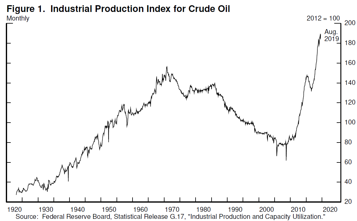
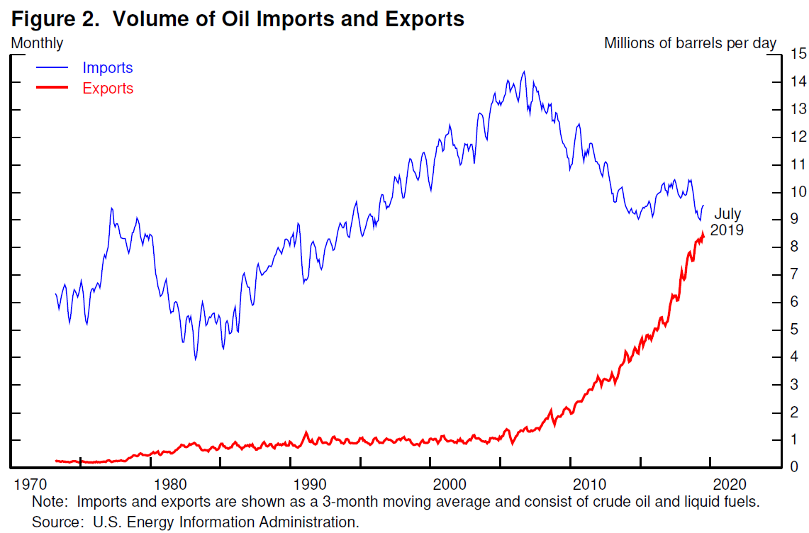
Let’s turn now to the first question of the consequences of an oil price spike. Figure 1 shows U.S. oil production since 1920. After rising fairly steadily through the early 1970s, production began a long period of gradual decline. By 2005, production was at about the same level as it had been 50 years earlier. Since then, remarkable advances in the technology for finding and extracting oil have led to a rapid increase in production to levels higher than ever before.3 In 2018, the United States became the world’s largest oil producer.4 Oil exports have surged, imports have fallen (figure 2), and the U.S. Energy Information Administration projects that this month, for the first time in many decades, the United States will be a net exporter of oil.5
As monetary policymakers, we closely monitor developments in oil markets because disruptions in these markets have played a role in several U.S. recessions and in the Great Inflation of the 1960s and 1970s. Traditionally, we assessed that a sharp rise in the price of oil would have a strong negative effect on consumers and businesses and, hence, on the U.S. economy. Today a higher oil price would still cause dislocations and hardship for many, but with exports and imports nearly balanced, the higher price paid by consumers is roughly offset by higher earnings of workers and firms in the U.S. oil industry. Moreover, because it is now easier to ramp up oil production, a sustained price rise can quickly boost output, providing a shock absorber in the face of supply disruptions. Thus, setting aside the effects of geopolitical uncertainty that may accompany higher oil prices, we now judge that a price spike would likely have nearly offsetting effects on U.S. gross domestic product (GDP).
How Should We Measure Output and Productivity?
Let’s now turn to the second question of how to best measure output and productivity. While there are some subtleties in measuring oil output, we know how to count barrels of oil. Measuring the overall level of goods and services produced in the economy is fundamentally messier, because it requires adding apples and oranges–and automobiles and myriad other goods and services. The hard-working statisticians creating the official statistics regularly adapt the data sources and methods so that, insofar as possible, the measured data provide accurate indicators of the state of the economy. Periods of rapid change present particular challenges, and it can take time for the measurement system to adapt to fully and accurately reflect the changes in the economy.
The advance of technology has long presented measurement challenges. In 1987, Nobel Prize—winning economist Robert Solow quipped that “you can see the computer age everywhere but in the productivity statistics.”6 In the second half of the 1990s, this measurement puzzle was at the heart of monetary policymaking.7 Chairman Alan Greenspan famously argued that the United States was experiencing the dawn of a new economy, and that potential and actual output were likely understated in official statistics. Where others saw capacity constraints and incipient inflation, Greenspan saw a productivity boom that would leave room for very low unemployment without inflation pressures. In light of the uncertainty it faced, the Federal Open Market Committee (FOMC) judged that the appropriate risk‑management approach called for refraining from interest rate increases unless and until there were clearer signs of rising inflation. Under this policy, unemployment fell near record lows without rising inflation, and later revisions to GDP measurement showed appreciably faster productivity growth.8
This episode illustrates a key challenge to making data-dependent policy in real time: Good decisions require good data, but the data in hand are seldom as good as we would like. Sound decisionmaking therefore requires the application of good judgment and a healthy dose of risk management.
Productivity is again presenting a puzzle. Official statistics currently show productivity growth slowing significantly in recent years, with the growth in output per hour worked falling from more than 3 percent a year from 1995 to 2003 to less than half that pace since then.9 Analysts are actively debating three alternative explanations for this apparent slowdown: First, the slowdown may be real and may persist indefinitely as productivity growth returns to more‑normal levels after a brief golden age.10 Second, the slowdown may instead be a pause of the sort that often accompanies fundamental technological change, so that productivity gains from recent technology advances will appear over time as society adjusts.11 Third, the slowdown may be overstated, perhaps greatly, because of measurement issues akin to those at work in the 1990s.12 At this point, we cannot know which of these views may gain widespread acceptance, and monetary policy will play no significant role in how this puzzle is resolved. As in the late 1990s, however, we are carefully assessing the implications of possibly mismeasured productivity gains. Moreover, productivity growth seems to have moved up over the past year after a long period at very low levels; we do not know whether that welcome trend will be sustained.
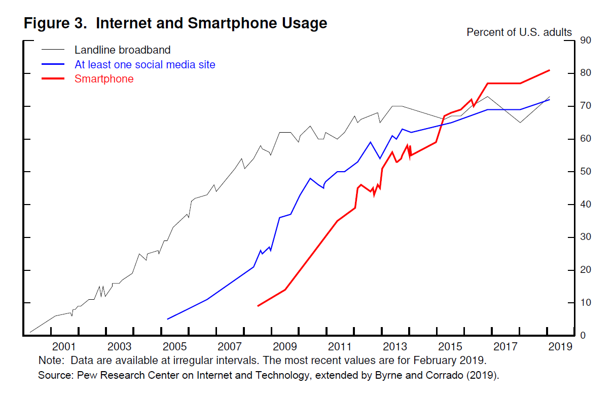
Recent research suggests that current official statistics may understate productivity growth by missing a significant part of the growing value we derive from fast internet connections and smartphones. These technologies, which were just emerging 15 years ago, are now ubiquitous (figure 3). We can now be constantly connected to the accumulated knowledge of humankind and receive near instantaneous updates on the lives of friends far and wide. And, adding to the measurement challenge, many of these services are free, which is to say, not explicitly priced. How should we value the luxury of never needing to ask for directions? Or the peace and tranquility afforded by speedy resolution of those contentious arguments over the trivia of the moment?
Researchers have tried to answer these questions in various ways.13 For example, Fed researchers have recently proposed a novel approach to measuring the value of services consumers derive from cellphones and other devices based on the volume of data flowing over those connections.14 Taking their accounting at face value, GDP growth would have been about 1/2 percentage point higher since 2007, which is an appreciable change and would be very good news. Growth over the previous couple of decades would also have been about 1/4 percentage point higher as well, implying that measurement issues of this sort likely account for only part of the productivity slowdown in current statistics. Research in this area is at an early stage, but this example illustrates the depth of analysis supporting our data-dependent decisionmaking.
How Tight Is the Labor Market?
Let me now turn from the measurement issues raised by the information age to an issue that has long been at the center of monetary policymaking: How tight is the labor market? Answering this question is central to our outlook for both of our dual-mandate goals of maximum employment and price stability. While this topic is always front and center in our thinking, I am raising it today to illustrate how we are using big data to inform policymaking.
Until recently, the official data showed job gains over the year through March 2019 of about 210,000 a month, which is far higher than necessary to absorb new entrants into the labor force and thus hold the unemployment rate constant. In August, the BLS publicly previewed the benchmark data revision coming in February 2020, and the news was that job gains over this period were more like 170,000 per month–a meaningfully lower number that itself remains subject to revision. The pace of job gains is hard to pin down in real time largely because of the dynamism of our economy: Many new businesses open and others close every month, creating some jobs and ending others, and definitive data on this turnover arrive with a substantial lag. Thus, initial data are, in part, sophisticated guesses based on what is known as the birth—death model of firms.
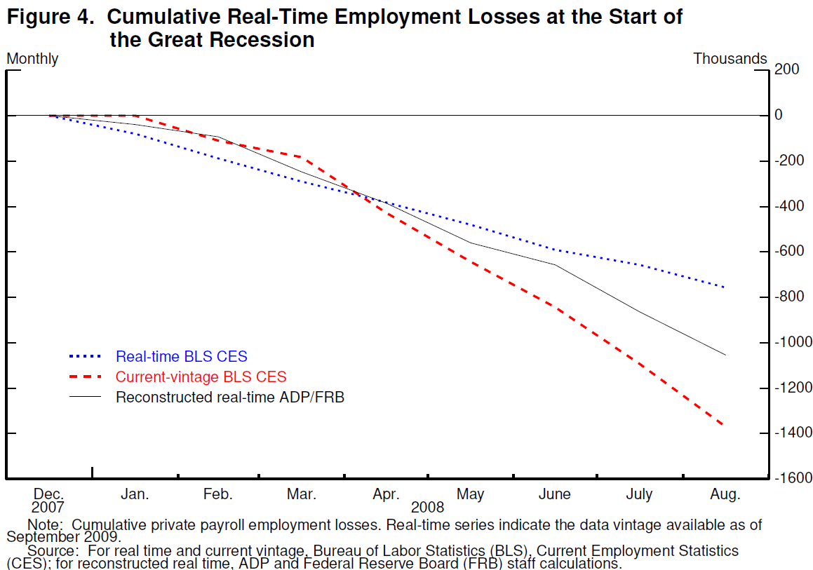
Several years ago, we began a collaboration with the payroll processing firm ADP to construct a measure of payroll employment from their data set, which covers about 20 percent of the nation’s private workforce and is available to us with a roughly one-week delay.15 As described in a recent research paper, we constructed a measure that provides an independent read on payroll employment that complements the official statistics.16 While experience is still limited with the new measure, we find promising evidence that it can refine our real-time picture of job gains. For example, in the first eight months of 2008, as the Great Recession was getting underway, the official monthly employment data showed total job losses of about 750,000 (figure 4). A later benchmark revision told a much bleaker story, with declines of about 1.5 million. Our new measure, had it been available in 2008, would have been much closer to the revised data, alerting us that the job situation might be considerably worse than the official data suggested.17
We believe that the new measure may help us better understand job market conditions in real time. The preview of the BLS benchmark revision leaves average job gains over the year through March solidly above the pace required to accommodate growth in the workforce over that time, but where we had seen a booming job market, we now see more-moderate growth. The benchmark revision will not directly affect data for job gains since March, but experience with past revisions suggests that some part of the benchmark will likely carry forward. Thus, the currently reported job gains of 157,000 per month on average over the past three months may well be revised somewhat lower. Based on a range of data and analysis, including our new measure, we now judge that, even allowing for such a revision, job gains remain above the level required to provide jobs for new entrants to the jobs market over time. Of course, the pace of job gains is only one of many job market issues that figure into our assessment of how the economy is performing relative to our maximum-employment mandate and our assessment of any inflationary pressures arising in the job market.
What Does Data Dependence Mean at Present?
In summary, data dependence is, and always has been, at the heart of policymaking at the Federal Reserve. We are always seeking out new and better sources of information and refining our analysis of that information to keep us abreast of conditions as our economy constantly reinvents itself. Before wrapping up, I will discuss recent developments in money markets and the current stance of monetary policy.
Our influence on the financial conditions that affect employment and inflation is indirect. The Federal Reserve sets two overnight interest rates: the interest rate paid on banks’ reserve balances and the rate on our reverse repurchase agreements. We use these two administered rates to keep a market-determined rate, the federal funds rate, within a target range set by the FOMC. We rely on financial markets to transmit these rates through a variety of channels to the rates paid by households and businesses–and to financial conditions more broadly.
In mid-September, an important channel in the transmission process–wholesale funding markets–exhibited unexpectedly intense volatility. Payments to meet corporate tax obligations and to purchase Treasury securities triggered notable liquidity pressures in money markets. Overnight interest rates spiked, and the effective federal funds rate briefly moved above the FOMC’s target range. To counter these pressures, we began conducting temporary open market operations. These operations have kept the federal funds rate in the target range and alleviated money market strains more generally.
While a range of factors may have contributed to these developments, it is clear that without a sufficient quantity of reserves in the banking system, even routine increases in funding pressures can lead to outsized movements in money market interest rates. This volatility can impede the effective implementation of monetary policy, and we are addressing it. Indeed, my colleagues and I will soon announce measures to add to the supply of reserves over time. Consistent with a decision we made in January, our goal is to provide an ample supply of reserves to ensure that control of the federal funds rate and other short-term interest rates is exercised primarily by setting our administered rates and not through frequent market interventions. Of course, we will not hesitate to conduct temporary operations if needed to foster trading in the federal funds market at rates within the target range.
Reserve balances are one among several items on the liability side of the Federal Reserve’s balance sheet, and demand for these liabilities–notably, currency in circulation–grows over time. Hence, increasing the supply of reserves or even maintaining a given level over time requires us to increase the size of our balance sheet. As we indicated in our March statement on balance sheet normalization, at some point, we will begin increasing our securities holdings to maintain an appropriate level of reserves.18 That time is now upon us.
I want to emphasize that growth of our balance sheet for reserve management purposes should in no way be confused with the large-scale asset purchase programs that we deployed after the financial crisis. Neither the recent technical issues nor the purchases of Treasury bills we are contemplating to resolve them should materially affect the stance of monetary policy, to which I now turn.
Our goal in monetary policy is to promote maximum employment and stable prices, which we interpret as inflation running closely around our symmetric 2 percent objective. At present, the jobs and inflation pictures are favorable. Many indicators show a historically strong labor market, with solid job gains, the unemployment rate at half-century lows, and rising prime-age labor force participation. Wages are rising, especially for those with lower-paying jobs. Inflation is somewhat below our symmetric 2 percent objective but has been gradually firming over the past few months. FOMC participants continue to see a sustained expansion of economic activity, strong labor market conditions, and inflation near our symmetric 2 percent objective as most likely. Many outside forecasters agree.
But there are risks to this favorable outlook, principally from global developments. Growth around much of the world has weakened over the past year and a half, and uncertainties around trade, Brexit, and other issues pose risks to the outlook. As those factors have evolved, my colleagues and I have shifted our views about appropriate monetary policy toward a lower path for the federal funds rate and have lowered its target range by 50 basis points. We believe that our policy actions are providing support for the outlook. Looking ahead, policy is not on a preset course. The next FOMC meeting is several weeks away, and we will be carefully monitoring incoming information. We will be data dependent, assessing the outlook and risks to the outlook on a meeting-by-meeting basis. Taking all that into account, we will act as appropriate to support continued growth, a strong job market, and inflation moving back to our symmetric 2 percent objective.
References
Brynjolfsson, Erik, Avinash Collis, and Felix Eggers (2019). “Using Massive Online Choice Experiments to Measure Changes in Well-Being,” Proceedings of the National Academy of Sciences, vol. 116 (April), pp. 7250—55.
Brynjolfsson, Erik, Daniel Rock, and Chad Syverson (2018). The Productivity J-Curve: How Intangibles Complement General Purpose Technologies. NBER Working Paper Series 25148. Cambridge, Mass.: National Bureau of Economic Research, October.
Bureau of Labor Statistics (2010). “Benchmark Article: BLS Establishment Estimates Revised to Incorporate March 2009 Benchmarks (PDF),” February 23.
––– (2019). “Introduction of Quarterly Birth/Death Model Updates in the Establishment Survey,” Current Employment Statistics, August 28.
Byrne, David M., and Carol Corrado (2019). “Accounting for Innovations in Consumer Digital Services: IT Still Matters (PDF),” Finance and Economics Discussion Series 2019-049. Washington: Board of Governors of the Federal Reserve System, June.
Cajner, Tomaz, Leland D. Crane, Ryan A. Decker, Adrian Hamins-Puertolas, and Christopher Kurz (2019). “Improving the Accuracy of Economic Measurement with Multiple Data Sources: The Case of Payroll Employment Data (PDF),” Finance and Economics Discussion Series 2019-065. Washington: Board of Governors of the Federal Reserve System, September.
Decker, Ryan, Aaron Flaaen, and Maria Tito (2016). “Unraveling the Oil Conundrum: Productivity Improvements and Cost Declines in the U.S. Shale Oil Industry,” FEDS Notes. Washington: Board of Governors of the Federal Reserve System, March 22.
Fernald, John G. (2015). “Productivity and Potential Output before, during, and after the Great Recession,” in Jonathan A. Parker and Michael Woodford, eds., NBER Macroeconomics Annual 2014, vol. 29. Chicago: University of Chicago Press, pp. 1—51.
––– (2018). “Is Slow Productivity and Output Growth in Advanced Economies the New Normal?” International Productivity Monitor, no. 35 (Fall), pp. 138—48.
Gordon, Robert J. (2017). The Rise and Fall of American Growth: The U.S. Standard of Living since the Civil War. Princeton, N.J.: Princeton University Press.
Hatzius, Jan, Zach Pandl, Alec Phillips, David Mericle, Elad Pashtan, Daan Struyven, Karen Reichgott, and Avisha Thakkar (2016). “Productivity Paradox v2.0 Revisited,” U.S. Economics Analyst, Goldman Sachs Economics Research, September 2.
Jorgenson, Dale W., Mun S. Ho, and Kevin J. Stiroh (2008). “A Retrospective Look at the U.S. Productivity Growth Resurgence,” Journal of Economic Perspectives, vol. 22 (Winter), pp. 3—24.
Powell, Jerome H. (2018). “Monetary Policy in a Changing Economy,” speech delivered at “Changing Market Structure and Implications for Monetary Policy,” a symposium sponsored by the Federal Reserve Bank of Kansas City, held in Jackson Hole, Wyo., August 23—25.
Rockoff, Hugh (2004). “Until It’s Over, Over There: The U.S. Economy in World War I,” NBER Working Paper Series 10580. Cambridge, Mass.: National Bureau of Economic Research, June.
Seskin, Eugene P. (1999). “Improved Estimates of the National Income and Product Accounts for 1959—98: Results of the Comprehensive Revision,” Survey of Current Business, vol. 79 (December), pp. 15—43.
Solow, Robert M. (1987). “We’d Better Watch Out,” New York Times Book Review, July 12.
U.S. Department of Energy (2018). “U.S. Becomes World’s Largest Crude Oil Producer and Department of Energy Authorizes Short Term Natural Gas Exports,” press release, September 13.
U.S. Environmental Protection Agency (2016). Hydraulic Fracturing for Oil and Gas: Impacts from the Hydraulic Fracturing Water Cycle on Drinking Water Resources in the United States, final report. Washington: EPA, December, available at http://cfpub.epa.gov/ncea/hfstudy/recordisplay.cfm?deid=332990.
1. Hugh Rockoff (2004) analyzes the change that accompanied a 44-month expansion starting in 1914. Return to text
2. For more information on the history of industrial production reporting at the Board, see “Celebrating 100 Years of the Industrial Production Index” at https://www.federalreserve.gov/releases/g17/100_years_of_ip_data.htm. Return to text
3. Decker, Flaaen, and Tito (2016) explore reasons for the resilience of production, even in light of declines in oil prices. Return to text
4. Department of Energy (2018). Return to text
5. The Energy Information Administration’s Short-Term Energy Outlook (STEO; available at https://www.eia.gov/outlooks/steo), released on September 10, 2019, shows that the United States will become a net exporter of crude oil and liquid fuels by October 2019. A new STEO will be published today. Return to text
6. Solow (1987). Return to text
7. I discuss and document this episode more fully in Powell (2018). Return to text
8. Revision and the role of high tech is described in Seskin (1999) and Jorgenson, Ho, and Stiroh (2008). Return to text
9. Between 1995 and 2003, business-sector output per hour increased at an annual rate of 3.4 percent, and it has risen only 1.4 percent since then. Fernald (2015) suggests 2003 as a break point for the beginning of the productivity slowdown. Return to text
10. See Gordon (2017) and Fernald (2018). Return to text
11. Brynjolfsson, Rock, and Syverson (2018). Return to text
12. Hatzius and others (2016). Return to text
13. In the case of Facebook, Brynjolfsson, Collis, and Eggers (2019) found that the median user required compensation of $48 to live without that social media platform for a month. Return to text
14. Byrne and Corrado (2019). Return to text
15. This share is comparable to that covered in the sample used by the BLS, but the BLS sample is designed to be representative, while the ADP sample is simply their customer base. Return to text
16. Cajner and others (2019). Return to text
17. Any example about the details of data deserves detailed comment. Our ADP-based estimate showed job losses of about 1 million over this period, considerably more than the real-time BLS data but well short of the post-benchmark value. This episode motivated the BLS to revise their procedures in ways that will reduce the revisions in similar episodes in the future. See BLS (2019) for a technical note last updated in August and BLS (2010). Return to text
18. See the Balance Sheet Normalization Principles and Plans, which are available on the Board’s website at https://www.federalreserve.gov/newsevents/pressreleases/monetary20190320c.htm. Return to text


So if it looks like a duck, swims like a duck, and quacks like a duck, why is then not a duck
“Neither the recent technical issues nor the purchases of Treasury bills we are contemplating to resolve them should materially affect the stance of monetary policy, to which I now turn.”
Why shouldn’t it
The invisible elephant in the room is also the trump budget, aka Fed deficit aka out-of-control multi-trillion insane spending, recently attached to a massive taxcut, which helped a few thousand millionaires and billionaires bur essentially steals money from the future.
One concept not discussed by anyone is that lower fiscal deficits “pull down” the Treasury yield, but instead, we have an insane president that wants to have a lower dollar, lower yields and a multi-trillion, increasing amont of debt that will once again, Destroy America.
In that light, here’s something grabbed fro space this morning:
“Nevertheless, the mid-September repo upheaval is a clear sign there might actually be limits on just how much debt the U.S. can take before triggering more frequent disruptions. Deficits aren’t exactly new, but they do add up. Since the crisis, the market for Treasury debt has roughly tripled in size.
And the fiscal balance has only gotten worse under President Donald Trump. The deficit surpassed $1 trillion in the first 11 months of the fiscal year, which just ended last month. And the Congressional Budget Office forecasts the shortfall this fiscal year will exceed $1 trillion. That all means the Treasury will need to keep increasing its debt auctions to fund the budget shortfalls.
“The Fed has shrunk its balance sheet in a meaningful way, resulting in reduced reserves in the system,” he said. The cash squeeze has “been further exacerbated by increased issuance, resulting in high levels of Treasury collateral settling into the market.”
Dealers aren’t getting as much help from foreign investors to soak up all that additional supply. Big creditors like China and Japan have slowed their buying of Treasuries in recent years. Overall, the share of foreign official holdings has shrunk to just over 25% this year, from a high of about 40% in 2008.
That waning appetite been reflected in the amount of bids investors submit versus the actual amount sold, known as the bid-to-cover ratio.
According to an analysis by John Canavan, Oxford Economics’ lead analyst, the ratio for 3-, 10- and 30-year debt sold each month has fallen to 2.39. That’s down from 2.89 times in January 2018, just before the Treasury began boosting its sales, and far lower than a high of 3.48 times in December 2011.
So-called auction tails, which occur when yields on debt issued at auction exceed prevailing levels in the market at the time of sale, have become more common as well. In layman’s terms, it’s a sign investors need to be paid more to take on new debt. That’s been true especially for longer-maturity debt, like the 10-year note and the 30-year bond.
“The debt has become more difficult to digest as the rise in Treasury issuance is outpacing the rise in demand, and overall there’s been a decline in recent years in foreign demand,” Canavan said.
There’s little to suggest the U.S. will suddenly decide to embrace fiscal restraint, either under Trump or a Democratic administration.
When it comes to financing America’s deficit though, it’s not the Fed that Julius Baer’s Markus Allenspach is worried about.
“There’s going to be saturation by investors at some point,” said Allenspach, head of fixed-income research and a member of the firm’s investment committee. “Yes, there is a global search for yield, but we believe we may be past the peak of this hunt for safe assets.””
https://www.fa-mag.com/news/repo-market-is-telling-washington-that-deficits-still-do-matter-52037.html?section=3&page=3
So basically we are just playing Japan and having the excess bonds being bought by the CB. Worked out great for them.
FYI, yet another take on BoneHeadMania:
Front-end pressures have been intensifying since the middle of last year,” Shahid Ladha, BNP’s head of G10 rates strategy, said in a market comment released late last week. “With small changes in demand for funding having large impacts on funding rates, we have reached the lowest comfortable level of reserves (LCLoR) at around $1.4 trillion. Structural collateral/liquidity imbalances result from the complex interaction of fiscal, monetary and macroprudential policy.”
Ladha sees several actions the Fed will be taking in the near-term.
“To maintain an ample reserves system and move clear of scarcity, we estimate the Fed needs to add nearly $400 billion of liquidity over the next year. The Fed is likely to shift balance sheet policy to formally target liabilities (from managing assets),” Ladha said.
“Since June 2018’s [interest rate on excess reserves] adjustment, the Fed’s response function to the growing collateral/liquidity imbalance has been reactive not proactive – necessary but not sufficient,” he wrote. “The N.Y. Fed successfully intervened with temporary open market repo operations.”
Ladha said that a bolder response was needed to keep control of front-end rates, maintain smooth U.S. Treasury auctions, limit contagion into other assets and reduce any undesired side effects into the banking system.
https://www.bondbuyer.com/news/sofr-so-good-as-issuance-keeps-on-growing-repo-tensions-not-anomaly
I like reading H style especially in articles like this. We also have some really good comment content to boot. Only online script I have!
Re: lowest comfortable level of reserves
Speech
Observations on Implementing Monetary Policy in an Ample-Reserves Regime
April 17, 2019
Lorie K. Logan, Senior Vice President
” … Third, the banking system’s demand for reserves could be higher than the sum of each bank’s individual demand if reserves are not distributed efficiently. This scenario could occur if there are financial market frictions to redistributing reserves that result in some banks persistently holding a surplus of reserves above their LCLoR. For example, banks now suggest that they face higher balance sheet costs to lend in federal funds, making it possible that this market would not be as efficient at redistributing reserves late in the day as it was prior to the crisis.18
These balance sheet costs can manifest themselves in less federal funds activity later in the day at rates near IOER. Prior to the crisis the federal funds market was liquid until late in the day. Banks could experience unanticipated late day outflows and still be confident in their ability to borrow from other banks holding excess reserves. Today, there is little late day activity in the federal funds market. As reserves decline and there is greater need to redistribute reserves, it is unclear if this activity will return as the opportunity cost of holding reserves is now lower. In the post-crisis era of super abundant reserves, bank lenders have largely left the federal funds market and today almost all lending is done by the Federal Home Loan Banks. In Desk outreach and the SFOS responses, many banks have indicated that rates would need to be well above IOER before the economics would be attractive enough to offset balance sheet costs that lending in the federal funds market incurs.
https://www.newyorkfed.org/newsevents/speeches/2019/log190417
Also see: (May 18, 2017) Fed officials originally said they planned to phase out their so-called reverse repo tool, initially introduced in 2013 to help the central bank maintain control over its benchmark federal-funds rate. The Fed said it would phase out the facility when it was no longer needed, but didn’t specify a time frame.
https://www.wsj.com/articles/fed-markets-lieutenant-suggests-reverse-repos-may-be-too-critical-to-phase-out-1495149437